Run FDTD and retain the computed port signals. These samples remain the direct simulation record.
MICROWAVE FDTD STUDIO / MULTIBAND GUIDEInside the guide.
Inside the guide.
Across the irises.
A two-dimensional section through the original waveguide simulation.
2D electric-field section · original solverMICROWAVE FDTD STUDIO / DUAL-MODE WAVEGUIDETwo modes.
Two modes.
One waveguide.
A clear two-dimensional section through the original dual-mode waveguide simulation.
2D field section · original solverMICROWAVE FDTD STUDIO / FOUR-POLE COAXFour resonators.
Four resonators.
Fields in focus.
A smooth cutaway of the four-pole filter without transmission zeros.
3D cutaway · collocated electric-field magnitudeMICROWAVE FDTD STUDIO / SIX-POLE COAXSix poles.
Six poles.
Two zeros.
Explore the original six-pole, two-zero filter through its computed fields.
3D cutaway · collocated electric-field magnitudeMICROWAVE FDTD STUDIO / NINE-POLE COAXNine poles.
Nine poles.
Three zeros.
A cutaway of the ninth-order filter reveals its recorded electric-field evolution.
3D cutaway · collocated electric-field magnitudeMICROWAVE FDTD STUDIO / SILVER-PLATED WAVEGUIDEInside the cavities.
Inside the cavities.
At 30 GHz.
Explore an original-solver electric-field section through the silver-plated waveguide geometry.
2D electric-field section · original solverMICROWAVE FDTD STUDIO / MICROSTRIP T JUNCTIONOne junction.
One junction.
Three ports.
Explore the computed electric field beneath a microstrip T junction.
3D Yee solver · recorded substrate field sectionMICROWAVE FDTD STUDIO / 4-BRANCH MICROSTRIPBranch by branch.
Branch by branch.
4 output branches.
Follow the computed substrate field through a branching microstrip demonstration model.
3D Yee solver · demonstration network · recorded field sectionMICROWAVE FDTD STUDIO / COUPLED-RESONATOR FILTERCoupled resonators.
Coupled resonators.
A different response.
Explore the computed field in a microstrip coupled-resonator filter demonstration.
3D Yee solver · demonstration filter · recorded field sectiont+
PREDICTIVE SIGNAL CONTINUATION
Predict the tail.
Shorten the simulation.
Resonant filters can keep ringing long after excitation. Microwave FDTD Studio uses the recorded port-signal decay to estimate its continuation, helping evaluate the frequency response without always waiting for the full tail to decay in the FDTD run.
Recorded transientPredicted decayFrequency-response comparison
Why the signal tail matters
Stopping a transient while appreciable energy remains can leave truncation ripples in a frequency-domain response. Signal continuation estimates the remaining decay from the acquired record, so its contribution can be included in the response calculation.
Fit the observed late-time behavior and extend the port response beyond the recorded interval. The continuation is predicted, not additional FDTD time steps.
Inspect the time-domain join and compare the frequency responses before and after estimation. Where provided below, the original exports show both views.
The practical advantage: a suitable, validated continuation can reduce the acquisition needed for slowly decaying resonant responses. The benefit depends on the structure, recording length and quality of the fit; these examples do not establish a universal speedup.
How to assess a predicted response
A smoother curve alone is not an accuracy test. Check prediction against withheld or longer recorded data, and check sensitivity to the fitting window and acquisition length. Grid convergence, port normalization, reference planes and losses still matter. Port-signal prediction does not extend spatial field volumes or generate new heat maps. Recorded and predicted results should be distinguished when reporting device performance.
MICROWAVE FDTD STUDIO · APPLICATION EXAMPLES
Explore the devices.
Ten waveguide, coaxial and microstrip examples. Open each model to inspect its original results.
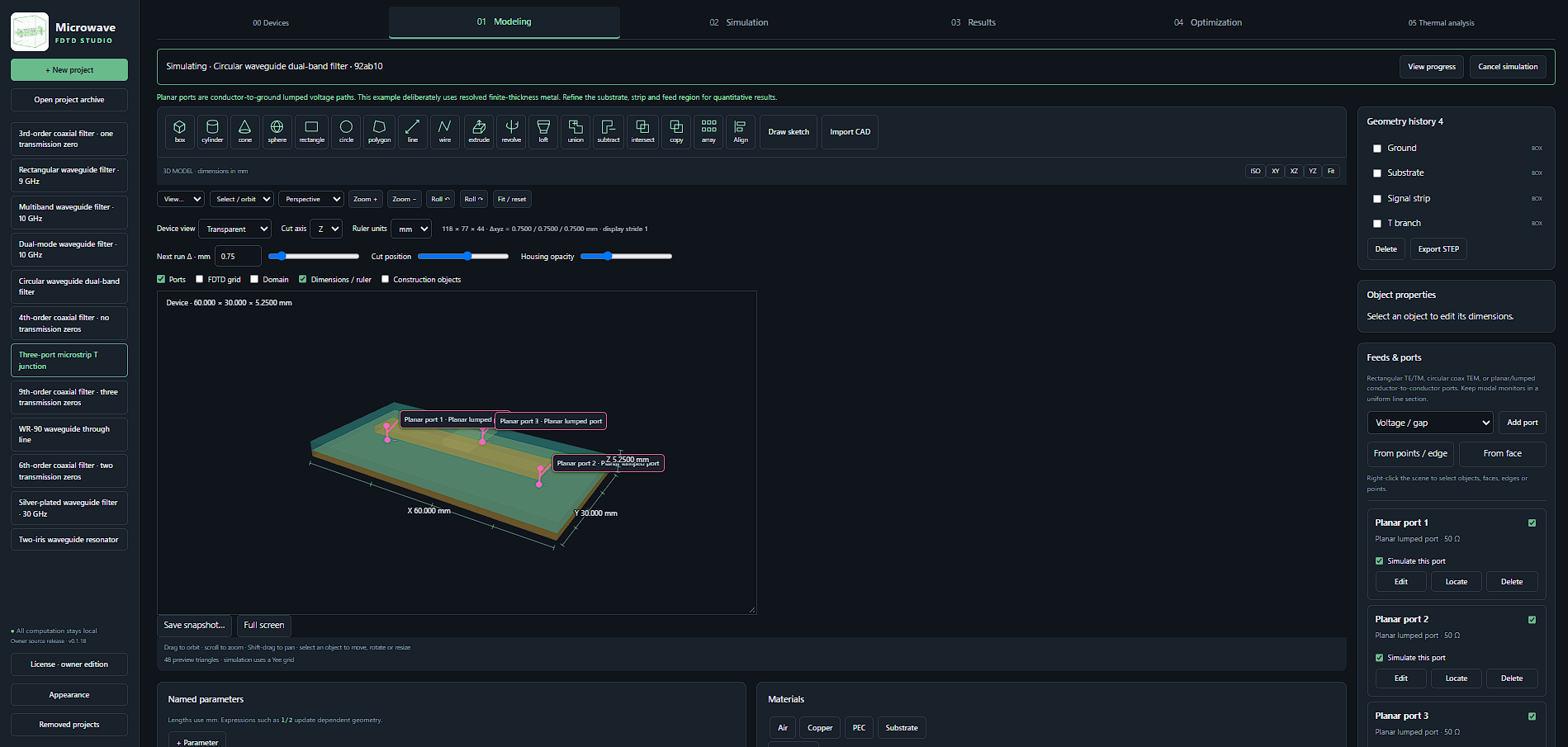
MICROWAVE APPLICATION
Three-port microstrip T junction
Geometry, recorded fields and exported device results.
Explore the example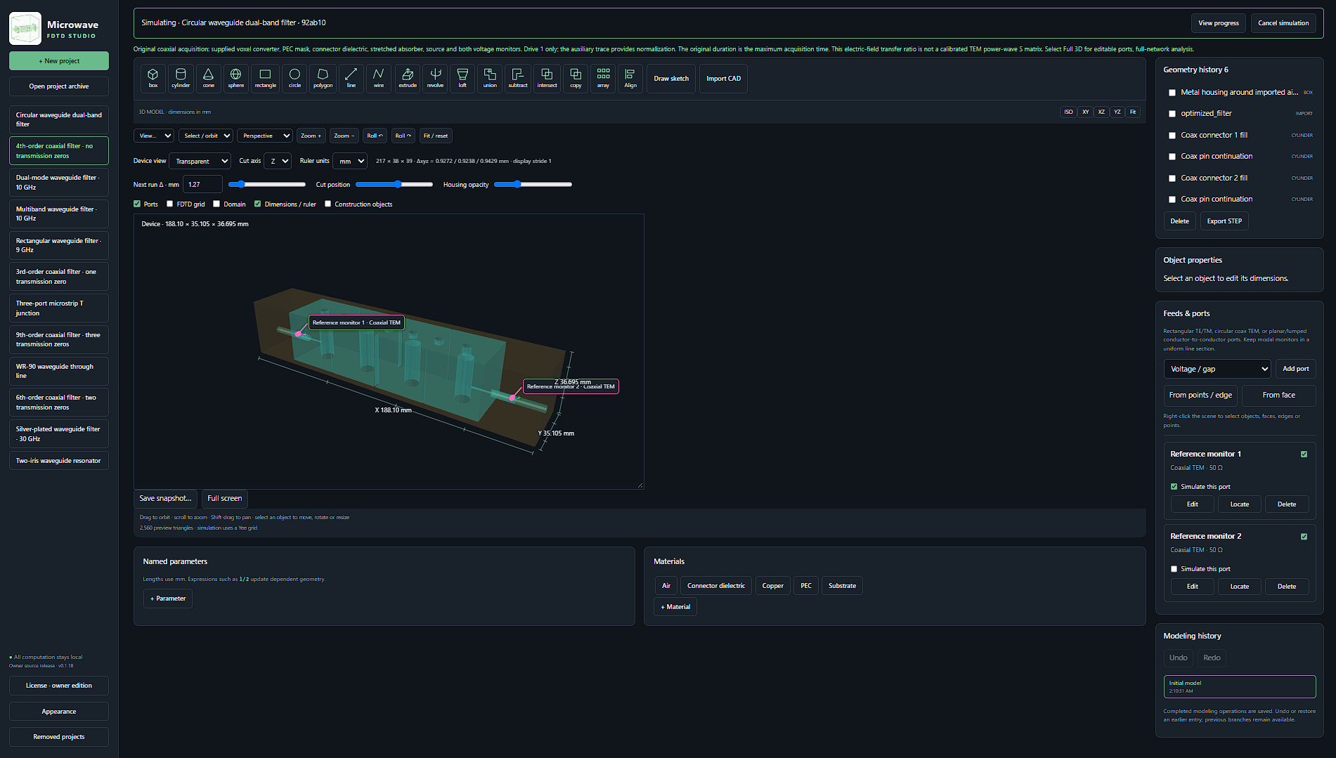
MICROWAVE APPLICATION
4th-order coaxial filter · no transmission zeros
Geometry, recorded fields and exported device results.
Explore the example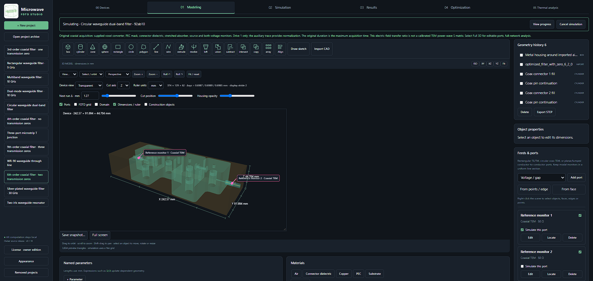
MICROWAVE APPLICATION
6th-order coaxial filter · two transmission zeros
Geometry, recorded fields and exported device results.
Explore the example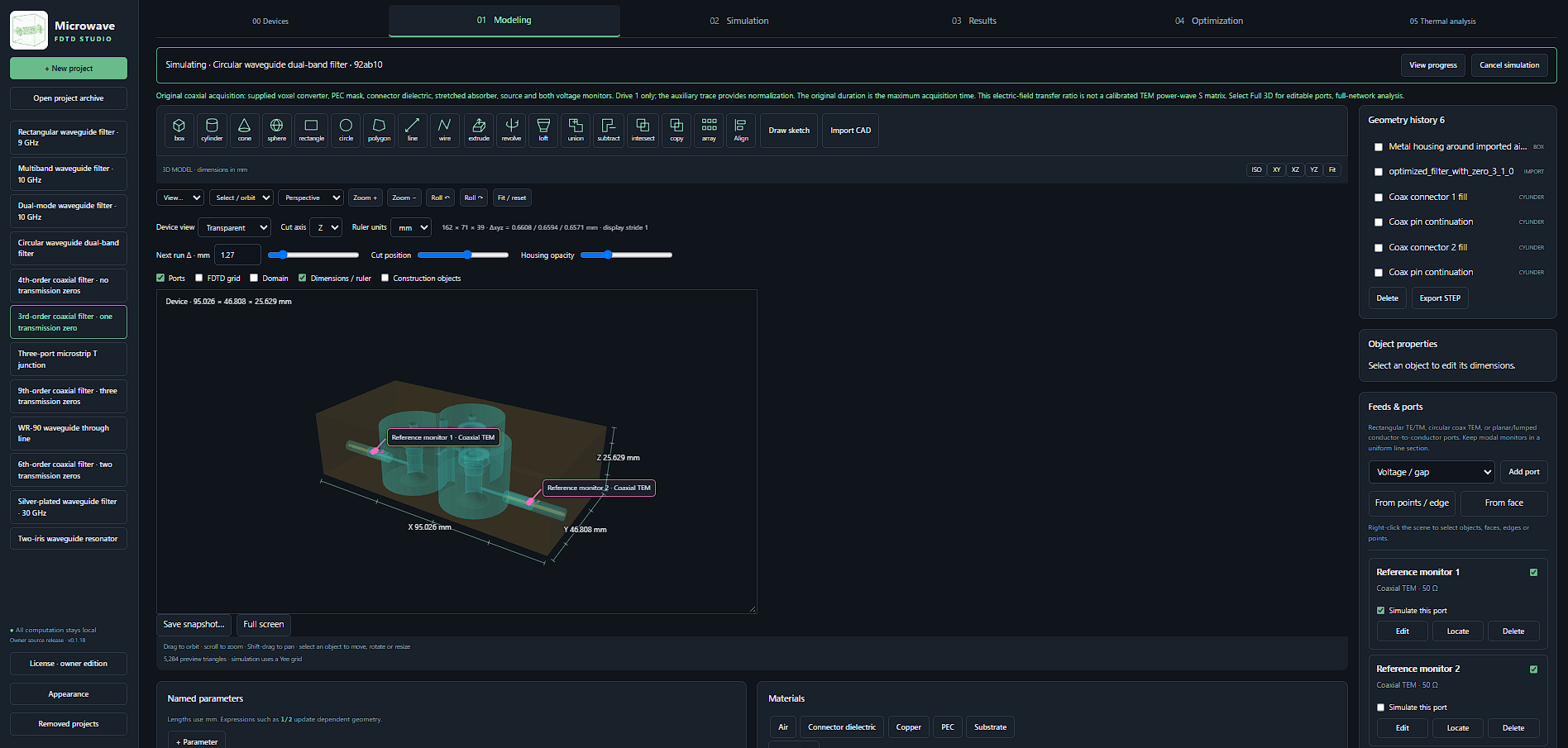
MICROWAVE APPLICATION
3rd-order coaxial filter · one transmission zero
Geometry, recorded fields and exported device results.
Explore the example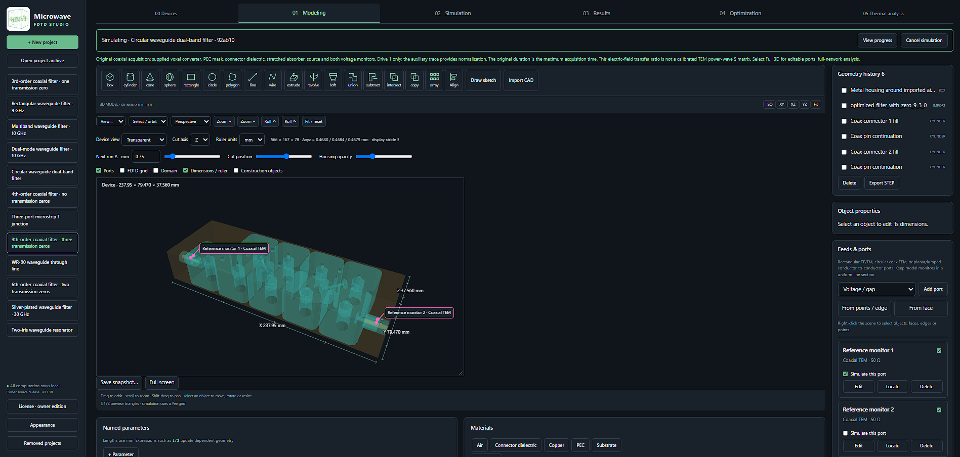
MICROWAVE APPLICATION
9th-order coaxial filter · three transmission zeros
Geometry, recorded fields and exported device results.
Explore the example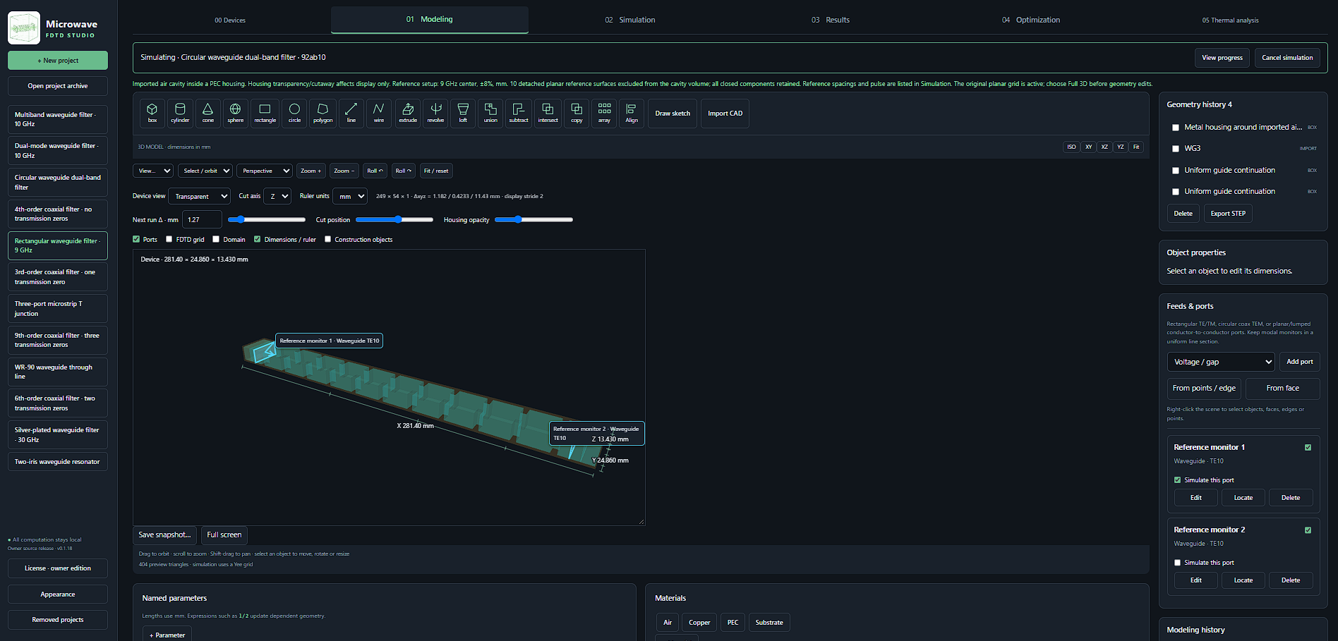
MICROWAVE APPLICATION
Rectangular waveguide filter · 9 GHz
Geometry, recorded fields and exported device results.
Explore the example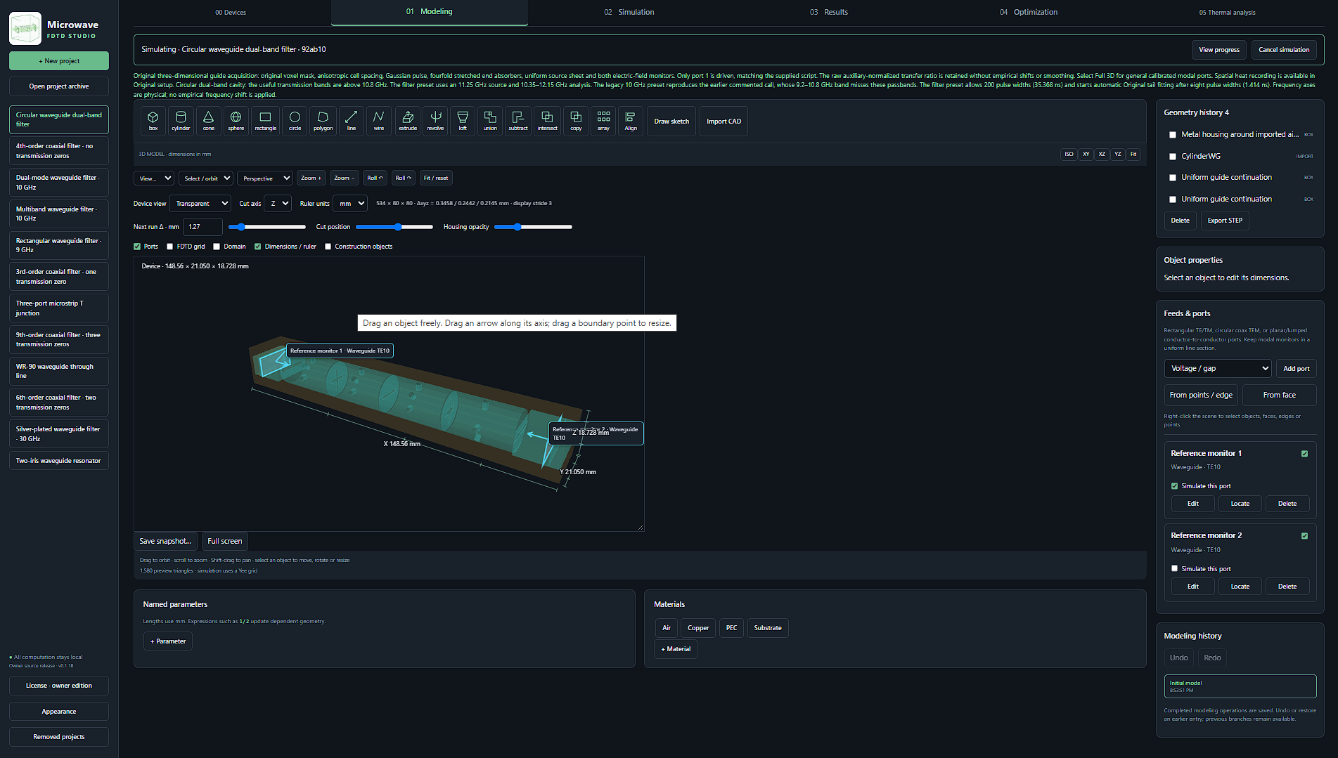
MICROWAVE APPLICATION
Circular waveguide dual-band filter
Geometry, recorded fields and exported device results.
Explore the example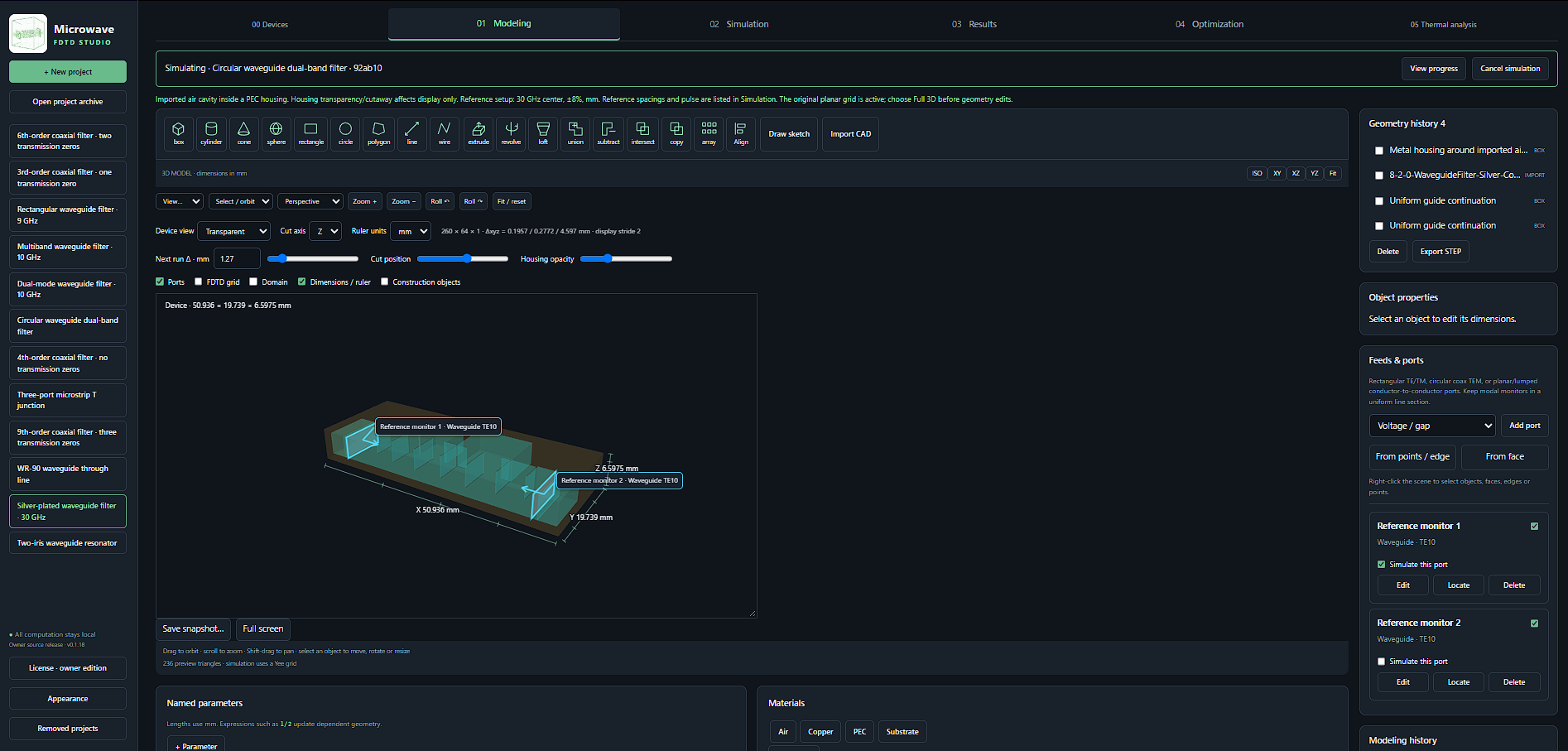
MICROWAVE APPLICATION
Silver-plated waveguide filter · 30 GHz
Geometry, recorded fields and exported device results.
Explore the example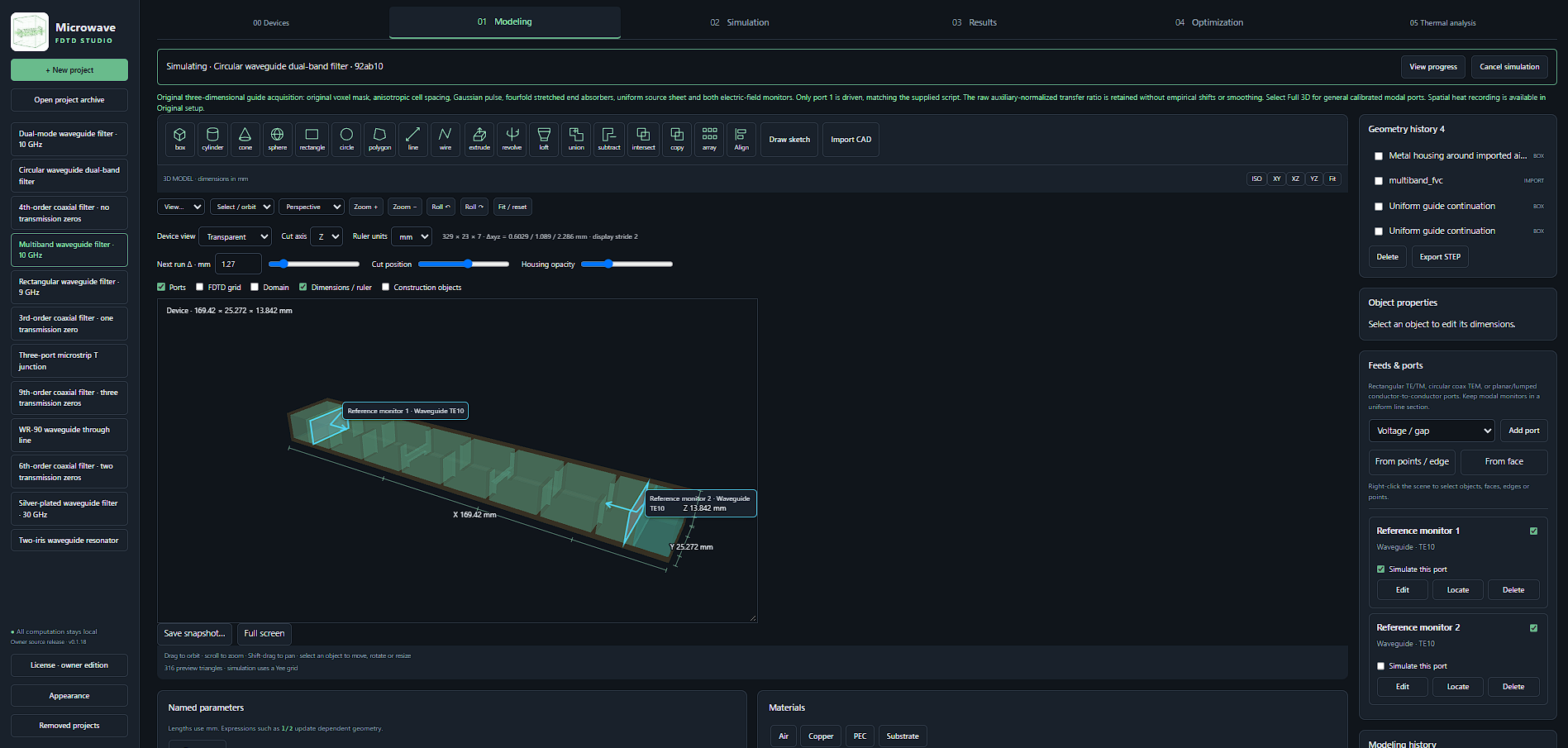
MICROWAVE APPLICATION
Multiband waveguide filter · 10 GHz
Geometry, recorded fields and exported device results.
Explore the example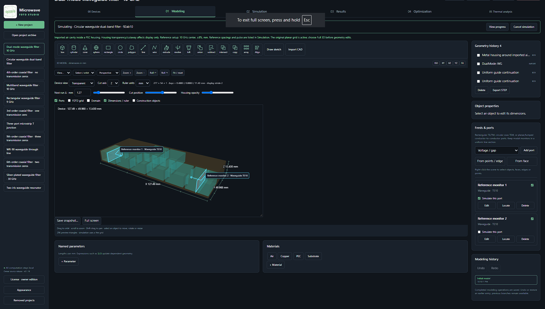
MICROWAVE APPLICATION
Dual-mode waveguide filter · 10 GHz
Geometry, recorded fields and exported device results.
Explore the exampleMICROWAVE FDTD STUDIO
From guided fields to device response.
01
Passive-device workflows
Explore filters, couplers and guided-wave structures in a workspace focused on microwave engineering.
02
Predictive port-signal continuation
Estimate the long-lived tail of port voltage and current responses from a shorter FDTD record. Check the continuation before using it in the response analysis.
03
Field inspection
Visualize field distributions to understand propagation, resonances and coupling within the structure.
04
Power-loss investigation
Explore electromagnetic loss and heat-estimation workflows, with attention to the assumptions and convergence of each model.
A FOCUSED WORKFLOW
Move from setup to understanding.
01
Choose a structure or template
02
Set materials, ports and boundaries
03
Run and check convergence
04
Inspect response, fields and losses
LET’S TALK ELECTROMAGNETICS
Have a problem you’d like to simulate?
Tell us about your geometry, frequency range and the results you need. Start a conversation about Microwave FDTD Studio and a suitable demonstration.
Connect with MohammadMohammad Marvasti · Founder of ComputeEM Studios and its software family
ALSO IN THE COMPUTEEM FAMILY
About these recorded fields
These fields come from complete runs of the original waveguide and coaxial solver equations on their original grids. The four earlier port records were compared with their bundled original baselines. The multiband and dual-mode waveguides use clean 2D sections; the four-pole, zero-free and six-pole, two-zero coaxial filters use CAD cutaways. Each earlier example has 160 recorded time samples. The silver-plated chapter uses the original lossless PEC model of that CAD geometry; it does not model finite-conductivity silver loss. The ninth-order, silver-plated and third-order chapters are additional captures from their original solver setups; they are not extra frames inferred from the exported demonstration videos. The final microstrip chapter shows a horizontal field section from a fresh run of the original three-port T-junction template. Contours are drawn from the recorded scalar fields, with a separate high-resolution CAD layer. DualMode-WG uses the original planar solver; the other examples use the original 3D grids. Coaxial magnitude views combine the three electric components only after Yee-to-cell-center collocation; waveguide close-ups show actual central cavities without stretching their geometry. These are recorded fields, not invented propagation; display selection and compression do not alter the retained raw results.