All Microwave examples
MICROWAVE FDTD STUDIO · APPLICATION EXAMPLE

4th-order coaxial filter · no transmission zeros

Explore the device model, recorded field evolution and original response exports in Microwave FDTD Studio.

01 · MODEL & PORTS

Model & ports
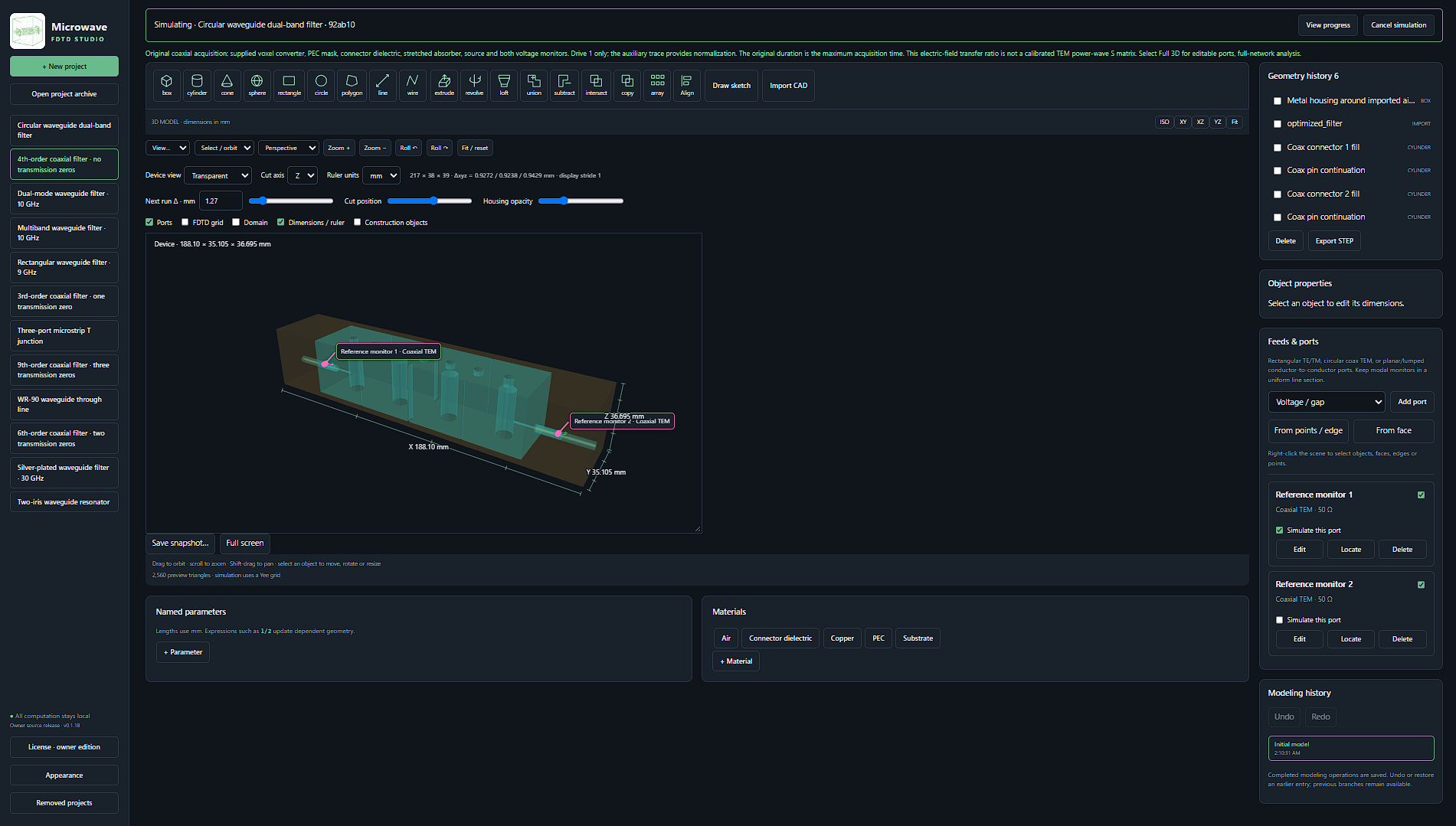
Microwave FDTD Studio modeling interface with 4th-order coaxial filter · no transmission zeros
Modeling workspaceOriginal modeling workspace showing the selected device, geometry and port setup.
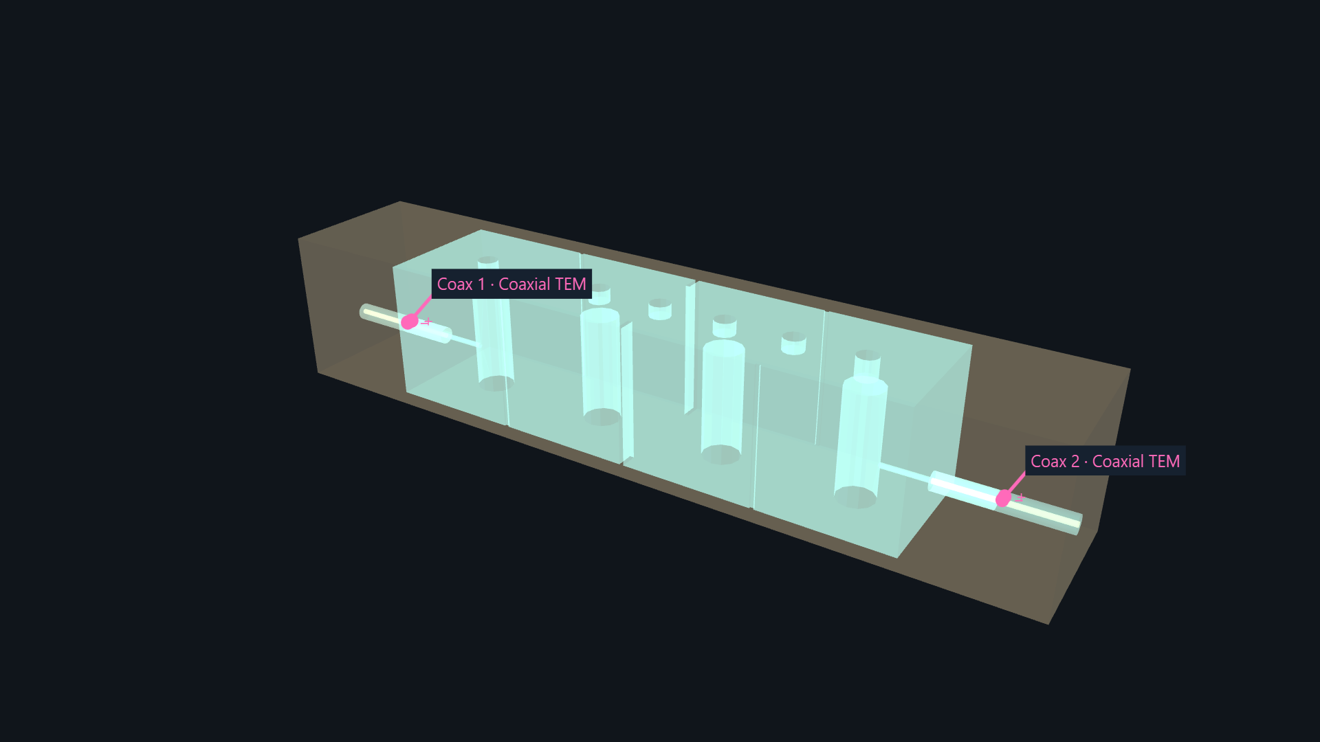
4th-order coaxial filter · no transmission zeros transparent model and labeled ports
Device geometryTransparent geometry with two labeled coaxial TEM ports and four inline resonators.
02 · RECORDED FIELDS

Recorded fields

Recorded EM-field slices show excitation spreading through the coupled resonators, followed by a changing stored-field pattern. Original 24 frames at 12 fps; playback time is not simulation runtime.

03 · TIME-DOMAIN SIGNALS

Time-domain signals

Inspect the excitation and decay in the original time-domain export. Port-signal continuation estimates the remaining tail from the acquired response; it does not add FDTD time steps. How predictive continuation works
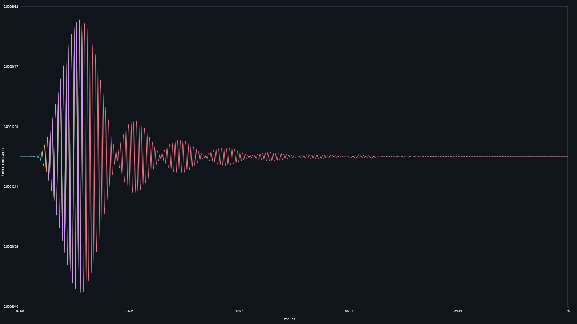
Electric-field overlap versus time for 4th-order coaxial filter · no transmission zeros
Time-domain port signalsOriginal time-domain electric-field overlap, showing the excited response and its decay. Read the time axis in nanoseconds; the continuation is estimated from the recorded port response.
04 · FREQUENCY RESPONSE

Frequency response
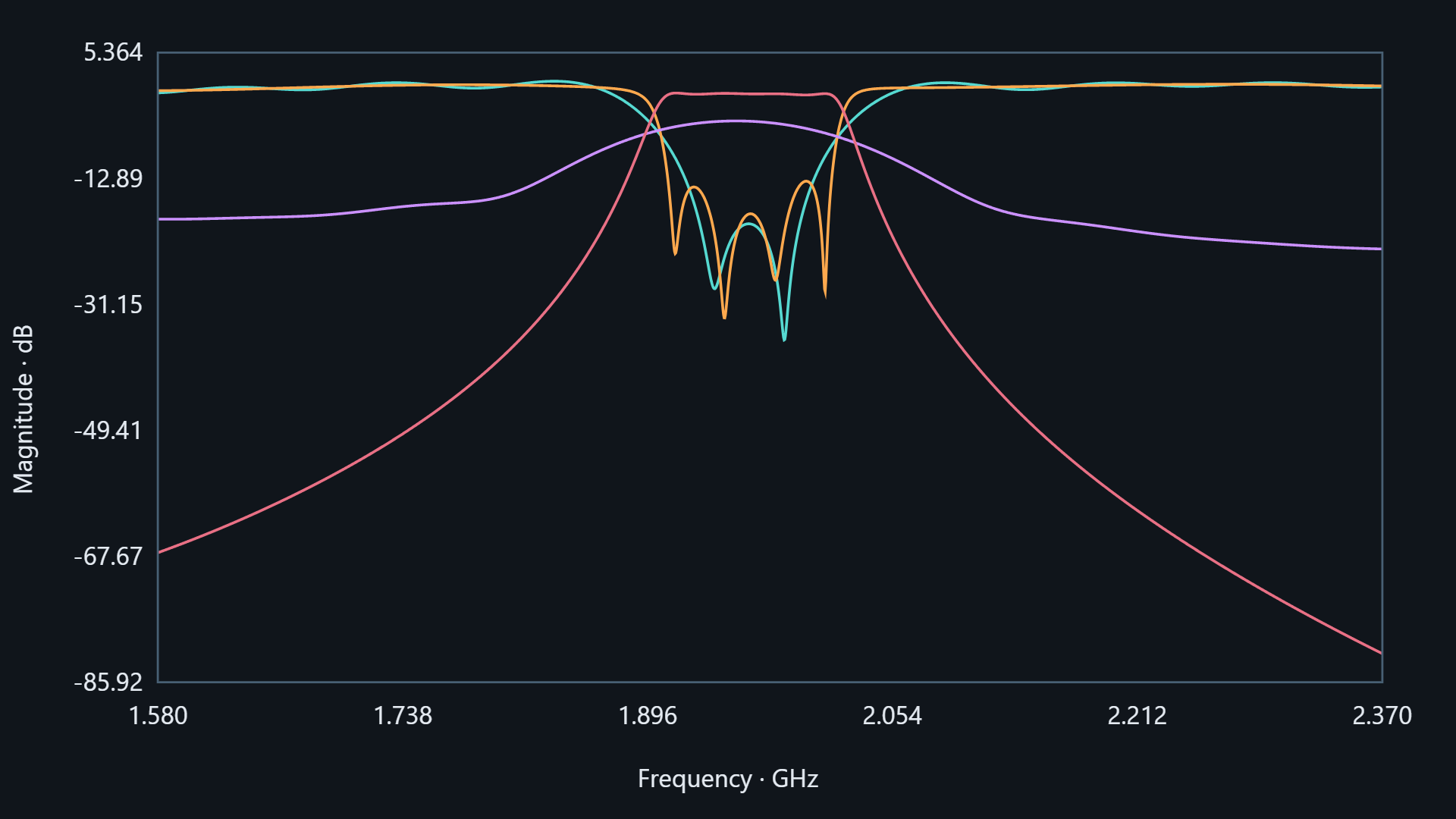
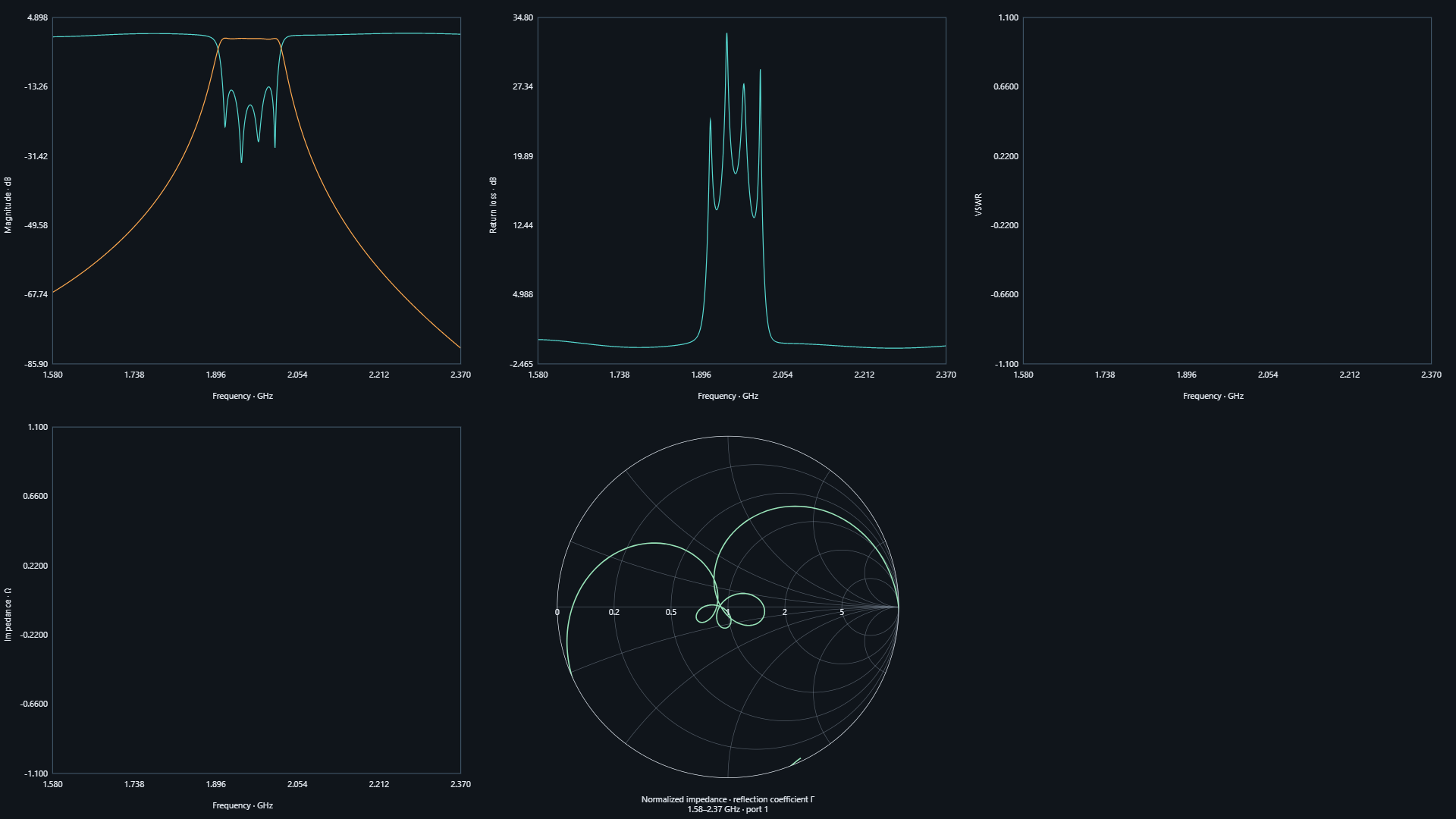
Magnitude in decibels versus frequency for 4th-order coaxial filter · no transmission zeros
Before and after signal estimationThe overlaid curves compare the response before and after signal estimation: the ripple-bearing trace is before estimation; the smoother trace is after estimation. The supplied axes and original trace colors are retained.
4th-order coaxial filter · no transmission zeros frequency response and impedance dashboard
Frequency-response overviewMagnitude, return-loss and normalized-impedance Smith-chart views across 1.58–2.37 GHz. The VSWR and impedance panels are empty; the acquisition caveat limits interpretation as calibrated S parameters.
05 · TEMPERATURE DISTRIBUTION

Temperature distribution

Spatial temperature results use the recorded electromagnetic load and thermal model. They are separate from port-signal prediction; compare numerical temperature scales rather than colors alone.
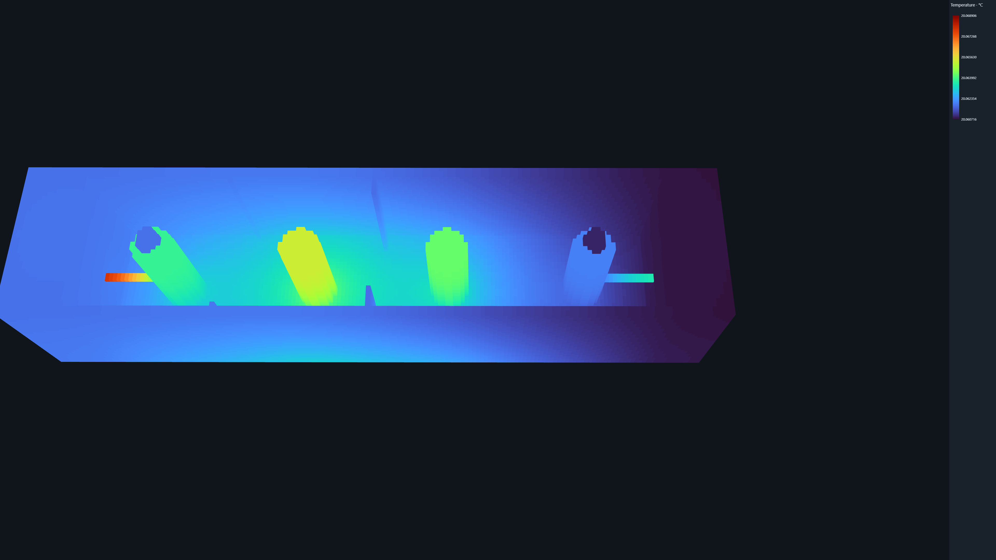
4th-order coaxial filter · no transmission zeros temperature distribution in degrees Celsius
Temperature distributionTemperature is mapped over the device geometry using the original °C scale. The image is a spatial temperature result, not a time trace or measured validation.
Result interpretation

Images preserve their original pixels, axes and color scales. Videos preserve source resolution and frame timing. These are recorded exports, not a live solver. The supplied acquisition uses auxiliary-normalized electric-field transfer ratios; these should not be read as a calibrated TEM power-wave S matrix.

Prediction quality requires checks against longer or withheld recorded data. A smoother curve alone does not establish accuracy or convergence.

Back to Microwave examples